Tamiĺs SPEW page
Warning: this page is pretty informal and not likely to change its attitude.
The Speciated Pollutant Emissions Wizard (SPEW) is a tool for calculating global emission inventories. Despite its origin, it isnĺt limited to inventories of particulate matter, but works on as many species as you provide data for. This page covers general SPEW operation, but not output.
Why SPEW?
I am an inventory developer by accident. I started out doing emission measurements and was trying to understand whether my results would have any impact on global emission inventories. I started with a four-line Excel spreadsheet and ended up with SPEW after a few years. The SPEW structure was developed because I got tired of trying to figure out why I had made certain decisions in the development of the emission inventory. Any inventory has plenty of (what I now label) ôWAGöŚwild-ass guesses. I later found that EPA uses the same terminology, but I hope they didnĺt trademark it, because I would owe them a lot of money. The trouble is that once your inventory is encoded, you canĺt remember how much of it is WAG, or where your ôgoodö data came from, unless you have a brain thatĺs way more organized than mine. I set up SPEW to provide traceable inventories and to allow quick re-running of inventories as new information came in and better decisions occurred. Any released data is tagged to an archived version number.
SPEW innards
SPEW files are .dbf (readable by dBase, FoxBase, Excel, etc.) The program itself uses a mix of SQL and dBase programming (whichever works faster or allows more flexibility). The reason I use dBase is the same as the reason so much modeling is done in FORTRAN: inertia. I happened to have some 12-year history with using dBase for business apps. I never could afford Oracle, and I donĺt much like Microsoft; Access feels like a ball-and-chain after dBase. Yes, I know hardly anyone else uses it and now I am stuck doing my own programming forever. After all this time, I find programming sort of mindless and relaxing, and if I only had time to relax...
Activity data
SPEW takes input from International Energy Agency data (for fossil fuels and biofuels). It can use United Nations data as well, although we prefer IEA data at this point. Weĺve also incorporated a number of ancillary activities, such as open biomass burning and urban waste burning, and ancillary breakdowns, such as state- or province-wise consumption of major fuels in large countries (U.S., China, India). Again, this is all automated and it is easy to add new breakdowns. Basically SPEW will use any data that has the format location-fueltype-flowtype-quantity, as long as you define the interface and the unit conversions. SPEW can lump whole sectors or pick out particular end-uses; but thatĺs only if country-specific end-use information is consistently available (and trustworthy). This part does not have a nice user interface yet. In fact, the encoding is fairly mystical (but completely traceable!).
It takes a few (~15) seconds to tabulate a yearĺs energy data, so doing time-trends is easy. Proofing the energy data, however, is another matter.
Emission information
The SPEW builder keeps track of the emission-characterization references. (These are put in under the ôReferencesö page, not shown here.) Then you can choose the emission factor (or other characteristic) you like the best. Tabulating these references is simple but time-consuming; identifying the good ones is not simple and still time-consuming. For this reason, every emission factor, for every region, and every data point in every reference is allowed a comment line.
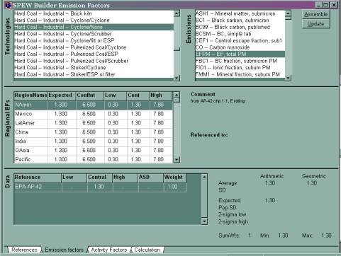
Features: StatsŚif you were lucky enough to have a lot of references for some source type, SPEW would calculate statistics of the expected values and confidence intervals. ôReferenced toöŚIf you have no emission info for a source type, you can set it up to automatically draw from some other source type. ôAssembleöŚsome emission factors have to be made by assembling PM emission factors plus speciation. These combinations are defined elsewhere and you can re-assemble the EF (and uncertainties) when you change the underlying information. For example: BC1, or submicron black carbon emission factor, is hardly ever measured. It is made from EFPM x FR1 (Submicron frac) x FBC1 (fraction BC) x CEF1 (fraction of particles escaping controls).
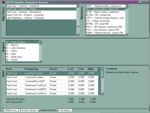
Activity factors
Each sector (like ôHard coalŚpower generationö) is divided into technologies that have different emission factors. This is how we account for practices in different regions.
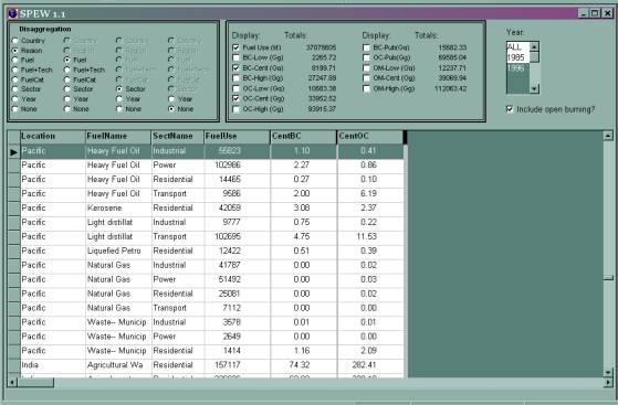
Slicing & dicing
This is the SPEW Viewer, which tabulates the results of the calculations, and will export them to ASCII files. A lot of disaggregation/aggregation is possible with this interface. You can choose the tabulations you want to show. (Hint: We do not believe the second decimal place.)
The emissions are gridded for atmospheric modeling with another interface, which is not very interesting and not shown here. Each fuel+sector is keyed to a gridding proxy, usually something to do with population or land use, but completely user-definable. For example, our open-burning agricultural emissions are gridded to (firecounts) x (fraction cropland). Currently we can do only 1-degree by 1-degree grids.
Uncertainties
SPEW supports my obsession with uncertainty. It keeps tabs on uncertainties in all the underlying factors (fuel use, emission factors, speciation etc.) and propagates them to global emissions. We can grid the uncertainties as well. The details are in our inventory paper. There are some subsidiary data-crunchers (not part of the interface) that sort out the major sources of uncertainty in each inventory.
Time Dependence
For our past and future inventory work, we've introduced time dependence of technology divisions. There's also a hierarchical activity builder which works from various proxies, choosing the best one. This was used for the Bond Group main page